1. The Question That Divided Physics
In 1935, three physicists — Albert Einstein, Boris Podolsky, and Nathan Rosen — published a paper that questioned whether quantum mechanics gave a complete description of physical reality. Their argument, now known as the EPR paradox, was elegant and devastating: if quantum mechanics were complete, then measuring one particle would instantaneously determine the state of its distant partner, what Einstein famously called "spooky action at a distance."
Einstein was not saying quantum mechanics was wrong. He was saying it was incomplete. Somewhere in the fabric of nature, he believed, there existed hidden variables — properties of particles that quantum theory simply did not account for, but which would restore determinism and locality to physics.
Niels Bohr disagreed. He argued that the quantum description was complete, and that particles simply do not possess definite properties until they are measured.
For nearly thirty years, this remained a philosophical debate. Then, in 1964, a physicist named John Stewart Bell — at the time a little-known researcher at CERN — showed that the debate was not philosophical at all — it was testable.
Bell derived a mathematical inequality that any theory based on local hidden variables must satisfy. Quantum mechanics, he showed, violates this inequality. The universe itself could be asked to choose sides — and it has. Repeatedly. For over fifty years of increasingly sophisticated experiments, nature has chosen the quantum side, decisively ruling out local hidden-variable theories.
This article walks through Bell's theorem from the ground up: the entanglement it describes, the inequality that bears his name, the experiments that confirmed it, and the profound — and often misunderstood — implications for our understanding of reality.
2. Quantum Entanglement Explained
Quantum entanglement is the phenomenon in which two or more particles become correlated in such a way that the quantum state of each particle cannot be described independently of the others, even when the particles are separated by large distances.
The Singlet State
The simplest entangled state is the spin singlet state of two spin-1/2 particles (such as two electrons, or — in Bohm's 1951 reformulation of EPR — the pair used throughout this article's math):
Here $|\uparrow\rangle$ and $|\downarrow\rangle$ represent spin-up and spin-down states measured along a chosen axis. The minus sign makes this an antisymmetric state — a singlet with total spin zero, the same mathematical form as EPR's original position/momentum entanglement, but for spin. The rest of this article works in spin-1/2 (Bohm) notation, which is the formulation Bell himself used.
Two Languages for One Physics: Spin vs. Polarization
The same physics is often written for photon polarization instead of electron spin. Photons are spin-1, so a rotation of an angle $\theta$ in the polarization plane corresponds to a rotation of $2\theta$ in the underlying spin space. That single difference is why you'll see both of these for the singlet-type correlation:
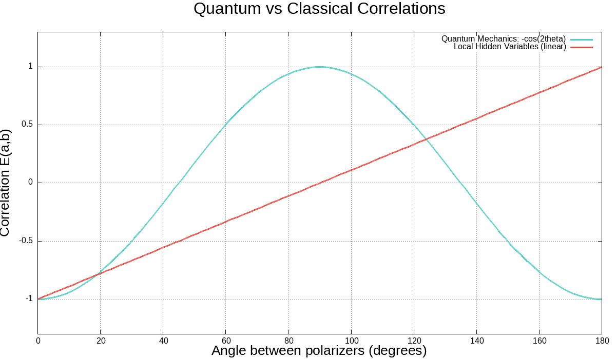
- Spin-1/2 (Bohm, used in this article's math): $\;E(\theta) = -\cos\theta$, where $\theta$ is the angle between the spin-measurement axes.
- Photon polarization (used in most experiments): $\;E(\theta) = -\cos 2\theta$, where $\theta$ is the angle between the polarizers.
Both curves violate Bell's inequality. They are the same phenomenon written in two bases — but the extra factor of 2 in the polarization version is a frequent source of confusion, so this article keeps the two straight from here on.
The key features of the singlet state:
Properties of the Singlet State
- Perfect anti-correlation: If Alice measures spin-up along any axis, Bob will measure spin-down along that same axis — with 100% certainty.
- No definite individual state: Neither particle has a defined spin along that axis before measurement. Each has a 50/50 chance of being up or down.
- Basis-independent: The anti-correlation holds regardless of which direction Alice and Bob choose to measure — as long as they measure along the same axis.
Correlation as a Function of Angle
When Alice and Bob measure along different axes, separated by angle $\theta$, quantum mechanics predicts the correlation:
where $E$ ranges from $+1$ (perfect correlation) to $-1$ (perfect anti-correlation), and $-\cos\theta$ comes directly from applying the spin operators to the singlet state. For photon polarizers at the same relative angle the equivalent result is $E(\theta) = -\cos 2\theta$, as noted in the box above.
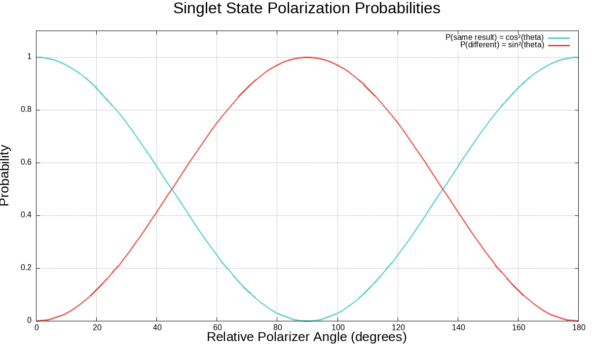
The same predictions in the polarization basis give the individual probabilities:
These predictions are counterintuitive but not obviously wrong — after all, correlation does not require faster-than-light communication in classical physics either (think of a pair of gloves mailed to different cities). The question is whether quantum correlations can be explained by any local, realistic theory. That is Bell's question.
3. The EPR Paradox: Einstein's Challenge
The 1935 EPR paper — "Can Quantum-Mechanical Description of Physical Reality Be Considered Complete?" — laid out a thought experiment that Einstein believed demonstrated quantum mechanics was incomplete. Here is the argument in outline:
The EPR Argument (1935)
Step 1: Two particles interact and then separate. Their combined quantum state is known (e.g., the singlet state).
Step 2: Alice measures her particle's position (or momentum, in the original). Because the state is entangled, she can immediately predict Bob's particle's position (or momentum) with certainty.
Step 3: Since Alice's measurement cannot instantaneously affect Bob's distant particle (the assumption of locality), Bob's particle must have had a definite position (momentum) all along.
Step 4: But quantum mechanics does not assign definite values to both position and momentum simultaneously (the uncertainty principle). Therefore, quantum mechanics does not describe all elements of physical reality — it is incomplete.
The two crucial assumptions in the EPR argument are:
The Two Pillars of Local Realism
Locality: A measurement performed here cannot instantaneously affect a physical system far away. Physical influences propagate at most at the speed of light.
Realism: Physical properties exist independently of measurement. The moon is there even when nobody looks.
Together, these form what physicists call local realism — the worldview that Einstein and most physicists took for granted.
Bohr's response was philosophical rather than mathematical. He argued that the very concept of an "element of reality" independent of the experimental context was meaningless in quantum mechanics. But without a way to test either view, the debate was unresolvable — until Bell.
4. Bell's Insight: From Philosophy to Testable Math
In 1964, John Stewart Bell was working at CERN, thinking about how to interpret quantum mechanics. He had read David Bohm's reformulation of the EPR argument using spin instead of position, and he asked a simple but revolutionary question:
If local hidden variables exist, what statistical predictions do they make? Can we derive a mathematical inequality that any local hidden variable theory must satisfy — and see whether quantum mechanics violates it? — In Bell's own words (paraphrased from his 1964 paper)
Bell's genius was realizing that hidden variables, however cleverly designed, are constrained by simple counting — just like the logic puzzles we solve in everyday life.
A Simple Analogy
Before the math, consider a concrete analogy. Imagine a factory that ships entangled pairs: Alice and Bob each receive one particle of a pair. On each run, Alice and Bob each choose randomly from a set of possible questions to ask their particle (for real spins, the direction of a measurement axis). Each question returns a $\pm 1$ answer.
Now suppose the particles are pre-programmed — the factory secretly slips each one a complete "answer booklet" giving the answer to every question it might ever be asked. The answer Alice's particle gives depends only on her question and the shared booklet, and Bob's answer depends only on his question and that same booklet. This "everything was decided in advance" idea is exactly the local hidden-variable assumption.
Here is the punchline: even with full freedom to fill in the booklets however you like, the answers to three questions $a$, $b$, and $c$ can never disagree enough to look like quantum mechanics. For any booklet, the three pairwise answers $A(a), A(b), A(c)$ satisfy a simple constraint — at most one of the three pairs can disagree. That constraint is Bell's inequality in disguise, and quantum mechanics breaks it. The factory analogy works for any classical, pre-programmed system but fails for quantum particles — and Bell proved this rigorously in the next section.

5. Deriving Bell's Inequality
Let's derive Bell's original inequality using Bohm's spin formulation. Consider a source that produces pairs of spin-1/2 particles in the singlet state. Alice measures spin along direction $\mathbf{a}$, and Bob measures along direction $\mathbf{b}$. Each measurement gives $+1$ or $-1$.
The Hidden Variable Model
A local hidden variable theory posits:
- There exists a hidden variable $\lambda$ (which could be a number, a vector, or even a complete description of the particle) that determines the outcomes.
- The outcome of Alice's measurement depends only on her setting $\mathbf{a}$ and $\lambda$: $A(\mathbf{a}, \lambda) = \pm 1$.
- The outcome of Bob's measurement depends only on his setting $\mathbf{b}$ and $\lambda$: $B(\mathbf{b}, \lambda) = \pm 1$.
- There is a probability distribution $\rho(\lambda)$ for the hidden variable, with $\int \rho(\lambda)\,d\lambda = 1$.
The correlation function predicted by any local hidden variable theory is:
The Inequality
Consider three measurement directions $\mathbf{a}$, $\mathbf{b}$, and $\mathbf{c}$. The whole argument rests on one counting fact. For any fixed value of the hidden variable $\lambda$, the outcomes $A(\mathbf{x},\lambda)$ and $B(\mathbf{y},\lambda)$ are each just $+1$ or $-1$. Now look at Bob's two possible answers, $B(\mathbf{b},\lambda)$ and $B(\mathbf{c},\lambda)$. Because each is $\pm 1$, their difference can only be $0$ (if the two answers agree) or $\pm 2$ (if they disagree). This single observation drives the rest of the proof.
A local hidden-variable theory must therefore satisfy, for every $\lambda$:
because the left side is $A(\mathbf{a},\lambda)\,[B(\mathbf{b},\lambda)-B(\mathbf{c},\lambda)]$, whose magnitude is $0$ when Bob's answers agree (right side $= 2 - 1 = 1$, and $0\le 1$) and $2$ when they disagree (right side $= 2 - (-1) = 3$, and $2\le 3$). Averaging over $\lambda$ with weight $\rho(\lambda)$:
Bell's original 1964 inequality is this same relation with the three settings relabelled (for example $|E(\mathbf{a},\mathbf{c}) + E(\mathbf{b},\mathbf{c})| \le 1 - E(\mathbf{a},\mathbf{b})$); all these forms are equivalent restatements of the one constraint: local, pre-existing answers cannot correlate the three measurement directions the way quantum mechanics does. In the modern form used by experiments, we repeat the argument with a fourth setting and add the two inequalities; the left-hand sides combine into the CHSH combination and the right-hand sides add to give the $|S|\le 2$ bound developed in Section 6. The essential point is unchanged: locality plus pre-existing outcomes force a bound on the correlations, and quantum mechanics exceeds it.
Key Result
Any theory based on local hidden variables must satisfy this inequality. This is not an assumption of quantum mechanics — it is a consequence of locality and realism alone. If experiments violate it, then at least one of those two assumptions must be false.
Quantum Mechanics Violates It
Quantum mechanics predicts for the singlet state:
where $\theta_{ab}$ is the angle between the measurement directions (the spin-1/2 result $E=-\cos\theta$ from Section 2; in the photon basis it is $E=-\cos 2\theta$). Now choose the three directions so that $\mathbf{a}$ and $\mathbf{b}$ are $90^\circ$ apart and $\mathbf{c}$ lies $45^\circ$ from each: $\mathbf{a}$ at $0^\circ$, $\mathbf{c}$ at $45^\circ$, $\mathbf{b}$ at $90^\circ$. The quantum correlations at these angles are:
Plug these into Bell's inequality in the form $|E(\mathbf{a},\mathbf{c}) + E(\mathbf{b},\mathbf{c})| \le 1 - E(\mathbf{a},\mathbf{b})$:
$1.414 > 1$ — the inequality is violated. Quantum mechanics predicts correlations that no local hidden-variable theory can reproduce. (This is the three-setting Bell inequality; Section 6 develops the four-setting CHSH form, whose quantum value $2\sqrt{2}\approx 2.828$ is the one experiments actually measure.)
6. The CHSH Inequality: The Form Experiments Use
Bell's original inequality used only one setting per observer. The form actually used in experiments was derived in 1969 by Clauser, Horne, Shimony, and Holt — the CHSH inequality. It uses two settings for each observer and is easier to test.
Setup
Alice chooses between settings $a$ or $a'$. Bob chooses between settings $b$ or $b'$. For each setting pair, they compute the correlation $E(a,b)$, etc. The CHSH quantity is:
For any local hidden variable theory:
Quantum mechanics predicts the maximum:
This maximum of $2\sqrt{2}$ is called the Tsirelson bound, after the mathematician Boris Tsirelson, who proved in 1987 that no quantum system can exceed it — a result that became a cornerstone of quantum information theory. It represents the absolute maximum violation allowed by quantum mechanics: nature violates the classical bound of 2, but stops short of the $4$ that is mathematically possible for a general theory (so "no-signalling" theories can, in principle, violate even further — quantum mechanics is not as extreme as nature could be).
Optimal Settings
The maximum violation is achieved when the measurement angles are:
| Observer | Setting | Angle |
|---|---|---|
| Alice | $a$ | $0^\circ$ |
| Alice | $a'$ | $45^\circ$ |
| Bob | $b$ | $22.5^\circ$ |
| Bob | $b'$ | $67.5^\circ$ |
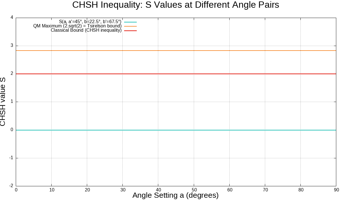
With these angles, quantum mechanics gives (using the photon correlation $E(\theta) = -\cos 2\theta$, where $\theta$ is the angle between the two settings):
The test uses $|S|$, so the sign is irrelevant: $|S_{\text{QM}}| = 2\sqrt{2} \approx 2.828$, the maximum quantum violation.
The Bottom Line
Measure $S$ in the lab. If $|S| > 2$, then local realism is false. Nature cannot be described by any theory in which particles have pre-existing properties and cannot influence each other faster than light.
7. The Experimental Verdict
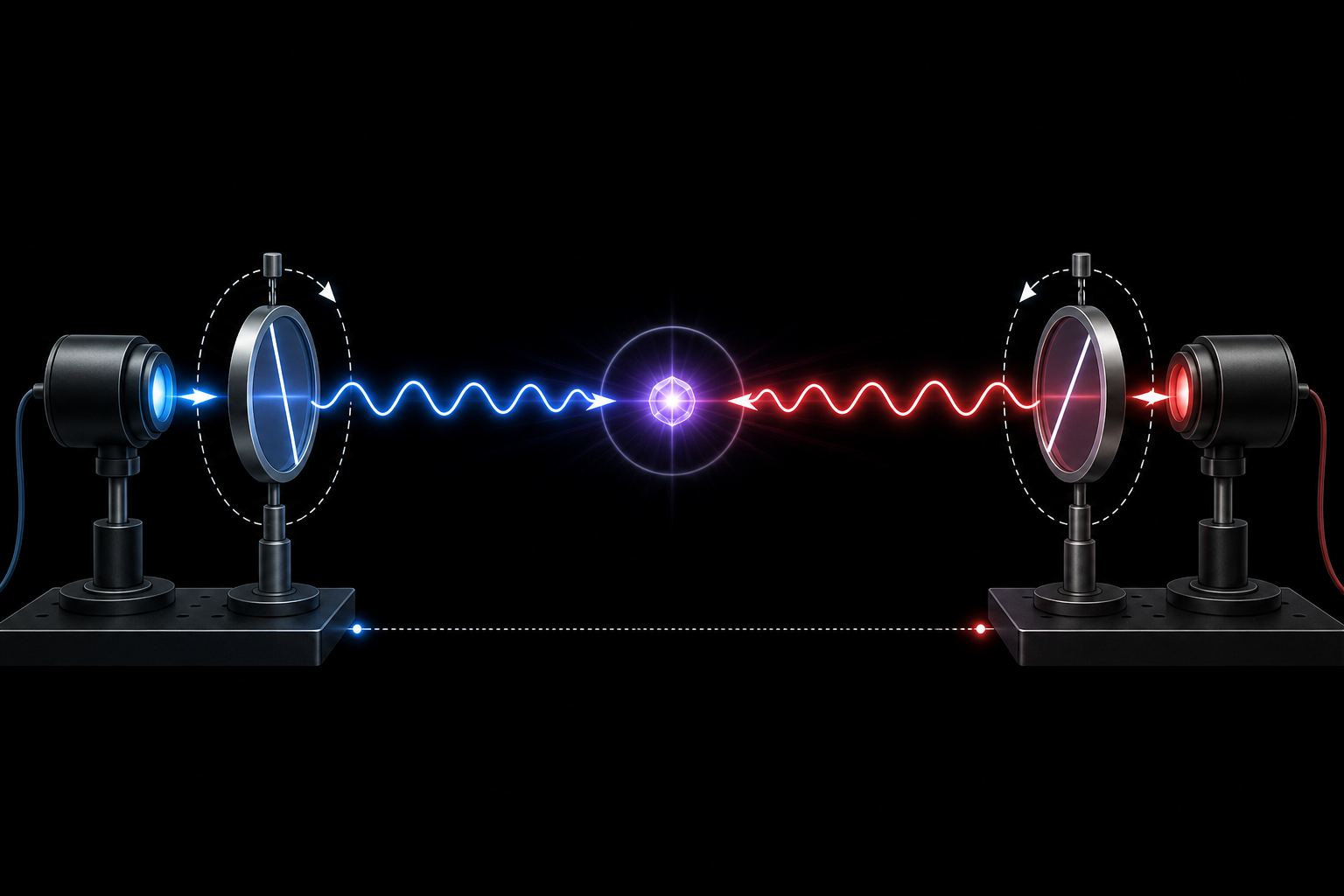
Bell's paper was published in 1964, but the technology to test it wasn't ready until the 1970s. The experiments have become increasingly sophisticated over five decades, closing loophole after loophole. The verdict has been consistent: quantum mechanics is correct; local realism is wrong.
Experimental Results at a Glance
| Year | Experiment | S Value | Classical Bound | Quantum Prediction |
|---|---|---|---|---|
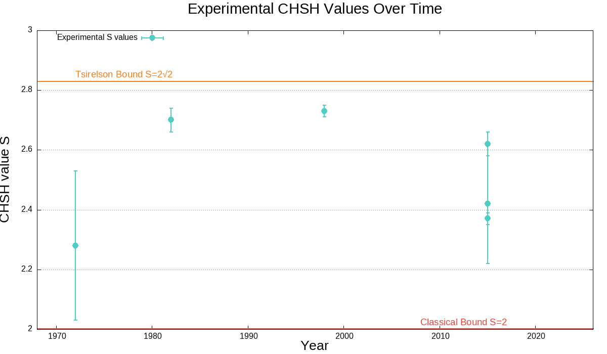
| 1972 | Freedman & Clauser | $\approx 2.28$ (raw) | 2.0 | $2.828$ |
| 1982 | Aspect et al. | $2.70 \pm 0.04$ | 2.0 | $2.828$ |
| 1998 | Weihs et al. | $2.73 \pm 0.02$ | 2.0 | $2.828$ |
| 2015 | Shalm et al. (NIST) | $2.37 \pm 0.02$ | 2.0 | $2.828$ |
| 2015 | Giustina et al. (Vienna) | $2.62 \pm 0.04$ | 2.0 | $2.828$ |
| 2015 | Hensen et al. (Delft) | $2.42 \pm 0.20$ | 2.0 | $2.828$ |
Every single experiment violates the classical bound of 2. The values cluster near the quantum mechanical prediction of $2\sqrt{2}$, with deviations attributable to experimental imperfections (detector efficiency, alignment errors, environmental noise).
Loopholes
Bell tests must contend with several "loopholes" — potential weaknesses in the experimental design that could, in principle, allow local hidden variable theories to survive:
| Loophole | Description | Status |
|---|---|---|
| Locality | Alice's and Bob's settings must be chosen fast enough that no light-speed signal can coordinate them. | ✓ Closed (1982, Aspect) |
| Detection | Detectors must be efficient enough that the detected sample is representative of all pairs. | ✓ Closed (2015, multiple) |
| Freedom-of-choice | Setting choices must be truly random and independent of the source (and of the hidden variable $\lambda$). | ✓ Addressed (2017–18, cosmic Bell tests) |
| Memory | The source or detectors might "remember" previous runs and adjust their behavior. | ✓ Closed by statistical analysis (Finetuning-free tests) |
By 2015, the locality and detection loopholes had been closed simultaneously. Then came the "cosmic Bell tests." In 2017, Handsteiner et al. used light from stars in the Milky Way — whose photons left their sources hundreds to thousands of years ago — to determine the measurement settings. In 2018, Rauch et al. went further, using light from high-redshift quasars — photons that left their sources billions of years ago (at redshift $z \sim 0.78$) — to set the measurement choices. Together, these tests push any possible common-cause conspiracy back to the early universe. One caveat worth stating plainly: these tests push the freedom-of-choice loophole far into the past, but they can never close it logically — a superdeterminist could always postulate a conspiracy reaching all the way back to the Big Bang. They make local realism not just untested but deeply implausible, but the last logical door can only be shut by a philosophical decision, not an experiment. Local hidden-variable theories are, for all practical purposes, dead.
8. Is It Faster-Than-Light Communication?
Here is the question most readers are asking: If measuring one particle instantly determines the state of its distant partner, does that mean information travels faster than light?
The answer is no. And this is the crucial point that separates physics from science fiction.
The No-Communication Theorem
Although entangled particles exhibit instantaneous correlations across any distance, no usable information can be transmitted through quantum entanglement. Alice cannot send a message to Bob by measuring her particle, because she has no control over what result she gets — she gets $+1$ or $-1$ randomly, with equal probability.
Why "Spooky Action" Doesn't Violate Relativity
Consider Alice and Bob, separated by a light-year, each holding one half of an entangled pair:
- Alice measures her particle. She gets "up" or "down" — completely random, 50/50.
- Bob measures his particle. He also gets "up" or "down" — also completely random, 50/50.
- Individually, both see random noise. Neither can tell what the other measured, or even whether the other measured.
- Only when they compare results (via a classical channel limited by the speed of light) do they see the correlation.
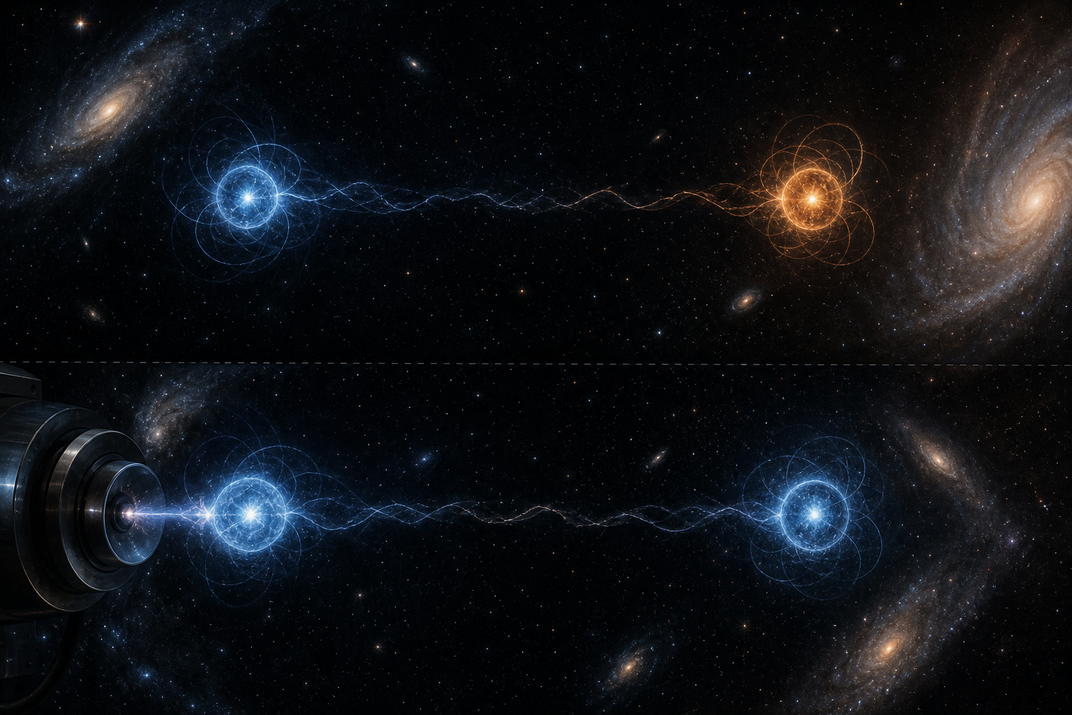
The correlation is real and instantaneous. But it carries no information by itself. To extract it, Alice and Bob must communicate classically — which is limited by $c$, the speed of light.
An Analogy: The Magic Coins
Imagine you have two special coins. You keep one and give the other to a friend who travels to Mars. Every time you flip your coin and get heads, your friend's coin also shows heads — even though the flip happened on Mars, light-minutes away.
Can you use this to send messages to Mars? No. Because you can't control whether your coin comes up heads or tails. Your friend just sees a random sequence of coin flips. Only when you call them on the phone (at light speed) and compare your sequences do you discover the perfect correlation.
This is exactly what happens with entangled particles. The "spooky action" is real, but it is not a communication channel. Special relativity is safe.
9. What It All Means: Interpretations
Bell's theorem tells us that local realism is false. But which part? There are several ways to interpret this, and physicists continue to debate which is correct:
Option A: Give Up Locality (Bohmian Mechanics)
In David Bohm's "pilot wave" interpretation, particles have definite positions at all times (realism is preserved), but they are guided by a non-local "quantum potential" that instantaneously connects all particles. Measuring one particle does instantaneously affect its partner — the non-locality is real and objective.
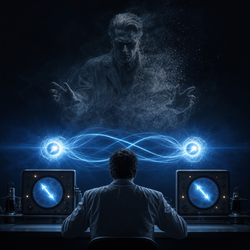
Option B: Give Up Realism (Copenhagen Interpretation)
In the Copenhagen interpretation (Bohr, Heisenberg), particles do not have definite properties before measurement. The wave function is the complete description of reality, and "measurement" is a fundamental process that creates definite outcomes. There is no spooky action because there is nothing to act — the properties don't exist until they are measured.
Option C: Many-Worlds (Everett)
In the many-worlds interpretation, both outcomes occur — in different branches of the universal wave function. When Alice measures "up," the universe splits: one branch where Alice sees up and Bob sees down, another where Alice sees down and Bob sees up. Correlation emerges from the structure of the wave function, not from any physical influence traveling between particles.
Option D: Retrocausality
A minority view suggests that measurement settings in the future can influence the particles' behavior in the past. This preserves locality but sacrifices our ordinary notion of causality. While logically possible, this view is not widely held.
Option E: Superdeterminism
If the universe is completely deterministic, then the "random" choices Alice and Bob make about measurement settings might have been correlated with the particles from the beginning of time. This preserves both locality and realism but at the cost of making science itself impossible — if everything is predetermined, experiments can't test anything.
| Interpretation | Locality | Realism | Cost |
|---|---|---|---|
| Bohmian | ✗ Lost | ✓ Kept | Non-local influences are real |
| Copenhagen | ✓ Kept | ✗ Lost | Properties don't exist until measured |
| Many-Worlds | ✓ Kept* | ✗ Lost | Universal wave function, branching worlds |
| Retrocausal | ✓ Kept | ✓ Kept | Future affects past |
| Superdeterminism | ✓ Kept | ✓ Kept | No free will, science is undermined |
*Many-worlds is technically local at the wave function level, but the branching structure is global.
Bell's theorem does not tell us which interpretation is correct — only that the world we live in is not the intuitively local, realistic world most of us expected. The universe is either non-local, non-real, or something stranger still. — Summary of the current consensus
10. Applications: Entanglement Powers Real Technology
Bell's theorem was once considered purely philosophical. Today, entanglement — the very phenomenon Bell helped us understand — powers an emerging technology revolution:
Quantum Cryptography (QKD)
Quantum Key Distribution uses entangled particles to generate encryption keys. If an eavesdropper tries to intercept the key, the act of measurement disturbs the entanglement and the violation of Bell's inequality disappears — revealing the intruder. This provides information-theoretic security, guaranteed by the laws of physics rather than the difficulty of mathematical problems.
Quantum Computing
Quantum computers use entangled qubits to perform computations that would take classical computers millions of years. Shor's algorithm for factoring, Grover's algorithm for search, and quantum simulation of molecular systems all rely on entanglement. The violation of Bell inequalities in quantum processors is actually a benchmark — it proves the device is genuinely quantum.
Quantum Teleportation
Not the sci-fi kind. Quantum teleportation uses entanglement to transfer the quantum state of a particle from one location to another, without the particle itself traveling. This is the foundation of the quantum internet — a network that connects quantum computers using entangled photon channels.
Device-Independent Security
The most recent application of Bell's theorem: "device-independent" quantum protocols. By verifying that a device violates Bell's inequality, you can certify that it is genuinely quantum — without needing to trust the manufacturer or understand the internal workings. This is security guaranteed by Bell's theorem itself.
From Philosophy to Industry
John Bell published his theorem in 1964 as a purely theoretical result. Today, companies sell quantum cryptography systems based on Bell-test principles, Google has demonstrated quantum supremacy using entangled processors, and the Chinese satellite Micius has performed entanglement distribution over 1,200 km. The "spooky action" that Einstein feared has become one of the most valuable resources in modern technology.
11. Conclusion: The Debate Is Settled
The question that divided Einstein and Bohr for decades has been answered by experiment. Nature does not obey local realism. Entangled particles are correlated in ways that no theory based on local hidden variables can explain.
But the answer is subtler than most pop-science accounts suggest:
- Entangled particles do not communicate with each other — there is no signal traveling between them, no violation of special relativity.
- They are not "connected" by an invisible wire. They are described by a single quantum state that exists across space — the state is fundamentally non-separable.
- The correlation is real and instantaneous, but it carries no information — it is a correlation, not a causation.
- The debate is not about whether particles "influence each other faster than light" — they don't. It's about whether physical properties exist independently of measurement — and the answer, Bell showed, is no.
John Bell gave us the tool to settle a question that had no experimental answer. And the answer changed our understanding of the universe: reality at its fundamental level is not local and not realist in the way our everyday intuitions suggest. Particles do not carry pre-existing instructions for every possible measurement. The act of measurement is not passive observation — it is an active process that participates in creating physical reality.
Einstein was wrong about his conclusion, but right about the question. It was a profound one, and it took a century of genius — from Bohr to Bell to Aspect to the Nobel laureates of 2022 — to answer it. The answer is that nature is stranger than we can suppose, and somehow, stranger than we should suppose.
There is no hope for any speculation that does not look absurd at first glance. — Niels Bohr
References
- Einstein, A., Podolsky, B., & Rosen, N. (1935). "Can Quantum-Mechanical Description of Physical Reality Be Considered Complete?" Physical Review, 47(10), 777–780.
- Bohm, D. (1951). Quantum Theory. Prentice-Hall. (Spin reformulation of the EPR argument.)
- Bell, J.S. (1964). "On the Einstein-Podolsky-Rosen Paradox." Physics Physique Физика, 1(3), 195–200.
- Bell, J.S. (1981). "Bertlmann's Socks and the Nature of Reality." Journal de Physique Colloques, 42(C2), C2-41–C2-62. (Also reprinted in Speakable and Unspeakable in Quantum Mechanics, Cambridge University Press, 1987. Accessible discussion of Bell's theorem; the famous "local causality" formulation.)
- Clauser, J.F., Horne, M.A., Shimony, A., & Holt, R.A. (1969). "Proposed Experiment to Test Local Hidden-Variable Theories." Physical Review Letters, 23(15), 880–884.
- Freedman, S.J., & Clauser, J.F. (1972). "Experimental Test of Local Hidden-Variable Theories." Physical Review Letters, 28(14), 938–941.
- Aspect, A., Grangier, P., & Roger, G. (1982). "Experimental Realization of Einstein-Podolsky-Rosen-Bohm Gedankenexperiment: A New Violation of Bell's Inequalities." Physical Review Letters, 49(2), 91–94.
- Weihs, G., Jennewein, T., Simon, C., Weinfurter, H., & Zeilinger, A. (1998). "Violation of Bell's Inequality under Strict Einstein Locality Conditions." Physical Review Letters, 81(23), 5039–5043.
- Tsirelson, B.S. (1987). "Quantum Generalizations of Bell's Inequalities." Lettere al Nuovo Cimento, 31(13), 331–344. (Proves the $2\sqrt{2}$ quantum bound.)
- Hensen, B., et al. (2015). "Loophole-Free Bell Inequality Violation using Electron Spins Separated by 1.3 Kilometres." Nature, 526, 682–686.
- Shalm, L.K., et al. (2015). "Strong Loophole-Free Test of Local Realism." Physical Review Letters, 115, 250402.
- Giustina, M., et al. (2015). "Significant-Loophole-Free Test of Bell's Theorem with Entangled Photons." Physical Review Letters, 115, 250401.
- Handsteiner, J., et al. (2017). "Cosmic Bell Test: Measurement Settings from Milky Way Stars." Physical Review Letters, 118(6), 060401.
- Rauch, D., et al. (2018). "Cosmic Bell Test Using Random Measurement Settings from High-Redshift Quasars." Physical Review Letters, 121(8), 080403. (Pushes the common-cause window back to redshift $z \sim 0.78$.)
- The Royal Swedish Academy of Sciences (2022). "The Nobel Prize in Physics 2022 — Press Release." NobelPrize.org. (Awarded to Aspect, Clauser, and Zeilinger.)